
Credits - Modelling and Risk

This article is about a modelling exercise on credits for students in secondary schools. Main goals are understanding of dynamics and identifcation of risks. Hence, we use a slightly modifed modelling cycle.
Índice
- Why credits and risks in math class?
- Why credits and risks in math classes?
- Starting point
- Starting point
- Assumptions, mathematical basics and goals
- Assumptions, mathematical basics and goals
- Modelling cycle
- Modelling cycle
- Deterministic model
- Deterministic model
- Deterministic model
- Probabilistic model
- Random exchange rate
- Random exchange rate and random interest rate
- Random exchange rate
- Random exchange rate and random interest rate
- Didactical comments
- Didactical comments
- Change of point of view
- References
- References
- Presentation
- Powerpoint
Why credits and risks in math classes?
Unfortunately, in Austria adolescents or young adults can't handle money in a decent[br]way. Some studies state that 14% of all visitors coming
firstly in contact with the debt[br]advice service are 25 years old or younger. Actually situations become worse by taking[br]a closer look, persons of not full age hardly seek advice at an official service institution.[br]They are used to ask their friends or parents for some
financial support. A smart-phone-[br]contract is the most common way for indebtedness in the youth, closely followed by a car[br]purchase. All these mentioned forms of borrowing money, even borrowing money from[br]your parents, are kinds of credits (see http://orf.at/stories/2208386/2208367/).[br]The author concentrates in his Ph.D.-thesis on
financial topics, which should be taught in[br]school, focus on secondary education. He creates central ideas of
financial mathematics[br]fundamental ideas in the sense of Bruner (see [2]) respectively, via an empirical study.[br]Three of these central ideas are "Use of stochastics in a
nance mathematical context",[br]"time value of money" and "handling of risk". The following modelling exercise is based[br]on these mentioned ideas.[br]The Austrian school curriculum stipulates the discussion of credits in class. Furthermore[br]in Austria there are some special schools, like "Handelsakademie" (commercial high-[br]school), which deal with credits in detail. However, all considerations in school are done[br]rather statically. Changes of the interest rate are rarely discussed.[br]In addition, in a bank consultation the assistant usually shows only one credit scenario[br]which is in favour of the debtor, though this is not the only possible scenario. From the[br]point of view of banks it is obvious, they want to realize profit. So, the credit user must[br]have such knowledge in such a consultation situation.[br]At this point we explicitly emphasize: We don't want to put the reader/resp. a pupil o
[br]raising a credit, but he/she should be able to understand the behaviour and the dynamics[br]of a credit and to be aware of its risks.
Starting point
We put ourself in the poor situation, we need money, lets say about 100 000 Euro, and[br]we haven't any other opportunity, except borrowing it. In the real world there are many[br]different types of loans. Before putting the signature on the right place of the contract,[br]we have to choose one credit. Which one will
fit perfectly? It's obvious, everybody tries[br]to get the best credit! Such a scenario allows many mathematical questions on different[br]intellectual levels, from school to research. Again, the article's focus is on secondary[br]education. We deduce the problem: "Which credit is the best?"
Assumptions, mathematical basics and goals
The process of modelling usually includes the translation of a real world problem to a[br]mathematical problem. We start the modelling cycle by giving assumptions:[br][list][*]We are credit-worthy for all appearing credits.[br][/*][*]There exist only four credits and one key interest rate p (think of Euribor):[/*][*][table][tr][td][b]Credit 1:[/b] The credit interest rate p[sub]1[/sub] equals the key interest rate p in every[br]interest rate period.[/td][/tr][tr][td][b]Credit 2:[/b] The credit interest rate p[sub]2[/sub] is 1% in the
rst period, 2% in the[br]second period and in the following periods p[sub]2[/sub] equals p.[/td][/tr][tr][td][b][/b][b]Credit 3:[/b] The credit interest rate p[sub]3[/sub] takes only values in a certain interval[br][2; 7]. If the key interest rate is below 2, then p[sub]3[/sub] equals 2 and if the key interest[br]rate is above 7, then p[sub]3[/sub] equals 7, otherwise p[sub]3[/sub] equals p.[/td][/tr][tr][td][b][/b][b]Credit 4:[/b] This credit is a foreign currency loan, particularly in Swiss franc.[br]We assume that this credit depends on the key interest rate p as well. In[br]the real world this is not the case, because one takes his debt in Swiss franc,[br]so the credit interest rate has to depend on the Swiss-Libor. As expected,[br]the exchange rate is important on such forms of credits. We denote er as the[br]exchange rate which says how many Swiss franc we get for one Euro. We don't[br]distinguish between bid and ask price and assume er to be constant over the[br]lent term.[/td][/tr][/table][br][/*][*]For convenience the interest rate period is one year.[br][/*][*]The key interest rate is variable, but constant over the whole credit term.[br][/*][*]The value of the instalments, the annuities, is constant over the whole credit term[br]and accounts for 8 400 Euro. One pays such amounts in arrears. In other words,[br]at
first the debt level will be raised by interest rate and then it will be reduced by[br]paying the annuity amount.[br][/*][*]We neglect all kind of charges and taxes related to the borrowing.[br][/*][/list][justify][math][/math][/justify][justify]Now, we shortly introduce the most important mathematical tool for this article the[br]"repayment-equation" and assume that the reader knows the following equation very[br]well. We identify important variables and denote S for the start level of debt, S[sub]n[/sub] for[br]the debt level after n years, R for the yearly instalments and p for the value of the key[br]interest rate in percent. The recurrence relation for S[sub]n[/sub] is:[br][math]S_n=S_{n-1}\cdot\left(1+\frac{p}{100}\right)-R[/math][br][br]One finds an explicit version below:[br][math][br][/math][math]S_n=S\cdot\left(1+\frac{p}{100}\right)^n-R\cdot\frac{\left(1+\frac{p}{100}\right)^n-1}{\frac{p}{100}}[/math][/justify]Which criteria are needed to mark the best credit? One assumption assures the constancy[br]of the instalments over the whole credit term. Then it's almost obvious, the best credit is[br]the one with the shortest lent term. In the following we are going to simulate the process[br]of the four different credits. An interest rate of a credit depends on the key interest rate[br]p, so the value of p represents the essential feature and is the one to be modelled. The[br]modelling takes place in a GeoGebra applet. We start with deterministic and end up[br]with probabilistic considerations.
Modelling cycle
Figure 1
The process of modelling is well known. The main steps of the modelling cycle also appear in this slightly modified cycle, see
gure 1 (e.g. see[1]). In this case students rapidly start the modelling-[br]cycle by a real world problem, here "Which credit is the best?" They translate this into a mathematical statement: "The best credit is the one with the shortest lent term." Afterwards they implement the four credits in a GeoGebra-applet. In the next stage pupils observe the dynamics and try to
find coherences respectively. Following this, they should mathematically justify their observations. If the validation of the mathematical solutions brings some flaws to light, they have to start again the modelling cycle from the beginning. In this case special knowledge about credits is needed, so some stages have to be guided by the teacher.
Deterministic model
We have already worked our way through the
first two steps, so it remains to implement[br]the GeoGebra applet. In this model we quickly create two sliders in GeoGebra, one for[br]the key interest rate p and the other for the exchange rate er. In the spreadsheet-view[br]one calculates the yearly debt level for the four credits by using the recurrence relation[br](1). For Example in cell B1 one
nds the formula "=B2*(1+p/100)-8 400", analogous[br]calculations for credit 2 (pay attention to the
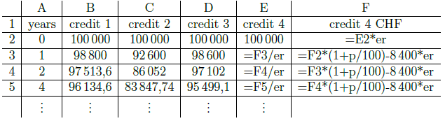
rst two periods!) and credit 3 (use if-[br]statements!). The calculations of credit 4, see table 1, lead to the same yearly debt levels[br]as for credit 1.
Table 1
We follow the idea of Heugl and create a list of points for every credit (see [3], p. 76).[br]The result is a nice visualization of the yearly debt levels of each credit. Different point[br]styles enable easy distinguishing between the four credits.
Figure 2.1
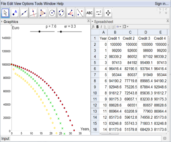
Figure 2.2
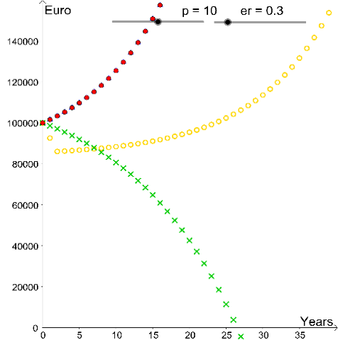
In school a stage of experiments might be of advantage, like manipulating slider bars[br]and observing its outcomes. In case of less experienced pupils the teacher should prepare[br]guiding questions, e.g. "What will happen, if the value of the key interest rate in-[br]creases/decreases?" or "At which values is credit 1 better than credit 2?" These heuristic[br]observations can be collected and shared in class.[br]Afterwards there is an opportunity to justify some of these
findings by using mathe-[br]matical argumentations. In this deterministic model one gets for every value of the key[br]interest rate p one best credit or for some values p two best credits, see below.
One gets such values by pairwise comparing the credits. For example one obtains 1.477[br]by using the equation (2) of credit 1 and 2 (slightly modified) and set S[sub]n[/sub] = 0. We express[br]the number of years n explicitly. In case of credit 1 we get per CAS (for convenience we[br]set q := 1 + p/100 ):
[math]n=\frac{ln\left(\frac{8400}{8400-\left(q-1\right)\cdot100000}\right)}{ln\left(q\right)}[/math]
[math]n=\frac{ln\left(\frac{q^2\cdot8400}{\left(1.02\cdot\left(q-1\right)+q\right)\cdot8400-1.01\cdot1.02\cdot\left(q-1\right)\cdot100000}\right)}{ln\left(q\right)}[/math]
We equal the two terms of the equations (3) and (4) and solve the resulting equation for[br]the variable q. Finally, we obtain q = 1.01477 and therefore p = 1.477.[br]In a validation of this model one will recognize some of its wrong results. It is impossible[br]that the yearly debt level of the foreign currency loan equals the yearly debt level of[br]credit 1. Empirical investigations like reading newspaper reveal this mistake in the model[br]above. Foreign currency loans have a bad press, actually in Austria they are forbidden[br]for hypothecary credits.
Random exchange rate
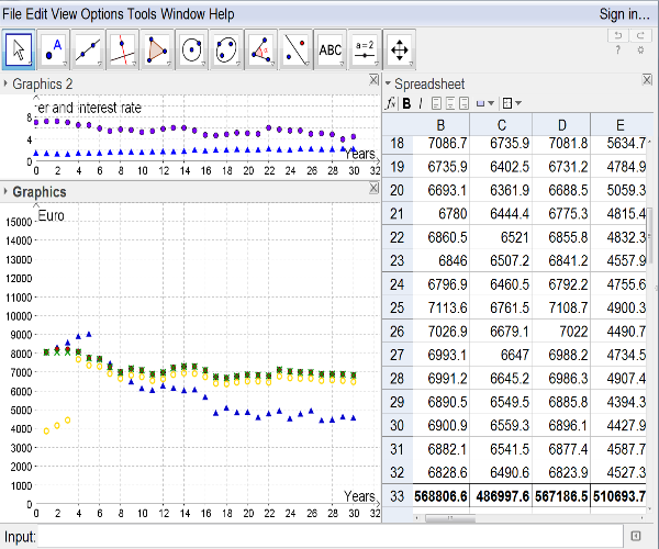
We improve our model, at
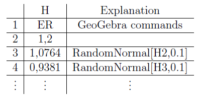
first we neglect the assumption about the constant exchange[br]rate. Now the exchange rate (er)n1 is a certain sequence. We start at time zero with[br]er[sub]0[/sub] = 1.2 and for the further periods we have er[sub]n+1[/sub] = er[sub]n[/sub]+X, where X is a random vari-[br]able with distribution N(0; 0,12) (In case of having not mentioned normal distribution[br]in class, one can use an equally distributed random variable instead). In the created Ge-[br]oGebra applet we slightly drop the slider bar about the exchange rate and construct the[br]mentioned sequence in the spreadsheet view, see Table 2. Furthermore we must change[br]the exchange rate er in column E and F according to random numbers in column H, e.g.[br]the command in cell F2 changes to "=E2*H2" and in F3 to "=F2*(1+p/100)-8 400*H3"
Table 2
We visualize the exchange rate sequence by small triangles in the view of graphics 2. The[br]pathways of the debt levels of the other credits are presented as before, see Figure 3.
Figure 3.1
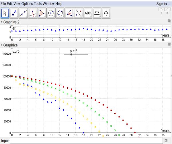
Figure 3.2
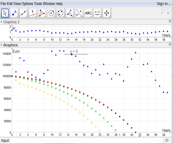
The creation of new scenarios easily happens by pressing the button F9 on the keyboard.[br]After creating this applet we are again in the stage of experiments in school. Guiding[br]questions, like "Which exchange rate paths are advantageous for the borrower (and which[br]aren't)?" lead pupils to the main focus.[br]Some coherences can be observed easily. A raise of the exchange rate is in favour of the[br]debtor (see left
gure 3) whereas a decrease of the exchange rate disadvantages the credit[br]user (see right
gure 3). Actually these heuristic observations require a proof.[br]A validation of the model above leads us to the point that the key interest rate can't[br]be constant over time. Its variations are the typical main source of the risk of a credit.[br]Again we try to model such an interest rate. The dilemma of raising a credit is the[br]variation of the key interest rate. One only knows the value of the interest rate for a[br]short term, here for the next year, in reality for the next three months. Then many[br]things affect the value of the key interest rate, like political, economic decisions and even[br]environmental happenings.
Didactical comments
The presented exercise basically includes different sequences of scholar activity like eventually collecting information about credits, setting up assumptions, creating the GeoGebra applet, observing dynamics and coherences, proving the observations under the formulated assumptions, revealing misbehaviour of the model. The use of the computer[br]is not restricted to creating an applet or observing dynamics, its application is proper[br]for almost every stage of the modelling cycle (see [4], p. 372), in particular: collecting[br]information in the internet and proving (e.g. using the CAS).[br]There are various application possibilities of this exercise in class: The teacher implements the whole exercise in class, including all modelling cycles as presented. Or, only[br]one modelling cycle is discussed in class. Or, only one credit is modelled in class e.g.[br]foreign currency loan. This exercise can be shortened (pupils' activity), in particular:[br]The teacher sets up such GeoGebra applets, pupils work on prepared guiding questions.[br]Or, there is no mathematical reasoning for the heuristic observations in class.[br]Wittmann suggests in the context of the "genetic principle" to change the point of view[br](see [5], p. 148
). As well one can do this in this exercise: We
fix the lent term to 30[br]years, and let the instalments vary. Then one receives the applet of figure 5:
Figure 5.1
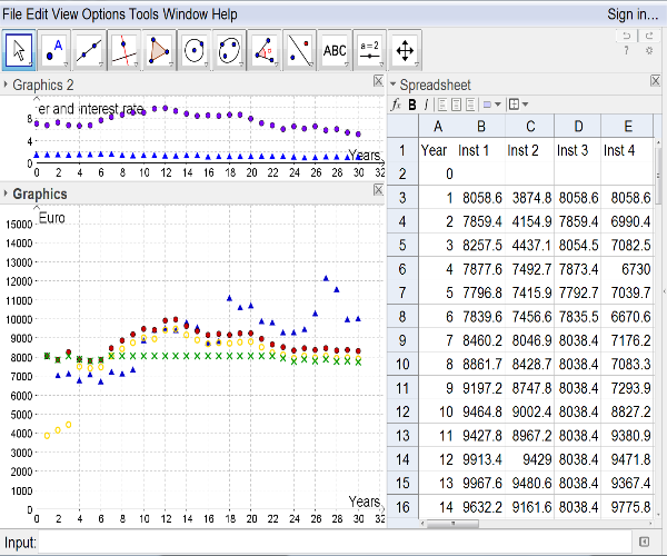
Figure 5.2
References
[1] Blum W. and Lei D., (2007) How do Students and Teachers deal with Modelling[br]Problems? In: Haines C. et al. (Eds): Mathematical Modelling (ICTMA 12): Edu-[br]cation, Engineering and Economics. Horwood, Chichester, pp. 222-231.[br][2] Bruner J., (1960) The process of education. Harvard University Press, Cambridge[br](Mass.).[br][3] Heugl H., (2014) Mathematikunterricht mit Technologie. Veritas, Linz.[br][4] Kaiser G. et al., (2015) Anwendungen und Modellieren. In: Bruder et al. (Eds):[br]Handbuch der Mathematikdidaktik. Springer, Wiesbaden, pp. 357-384.[br][5] Wittmann E., (2009) Grundfragen des Mathematikunterrichts (6. Ed.). Vieweg,[br]Braunschweig.