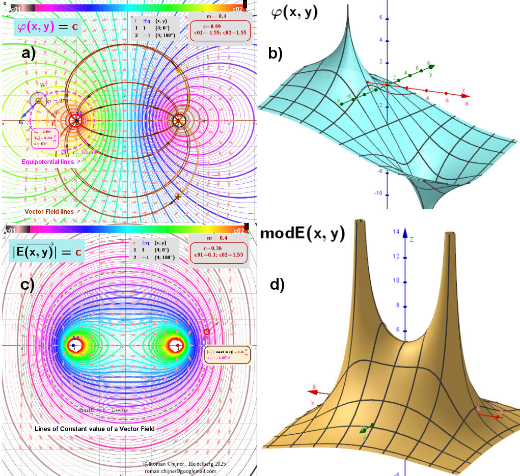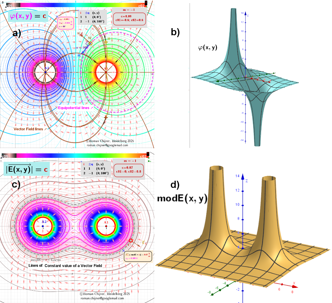
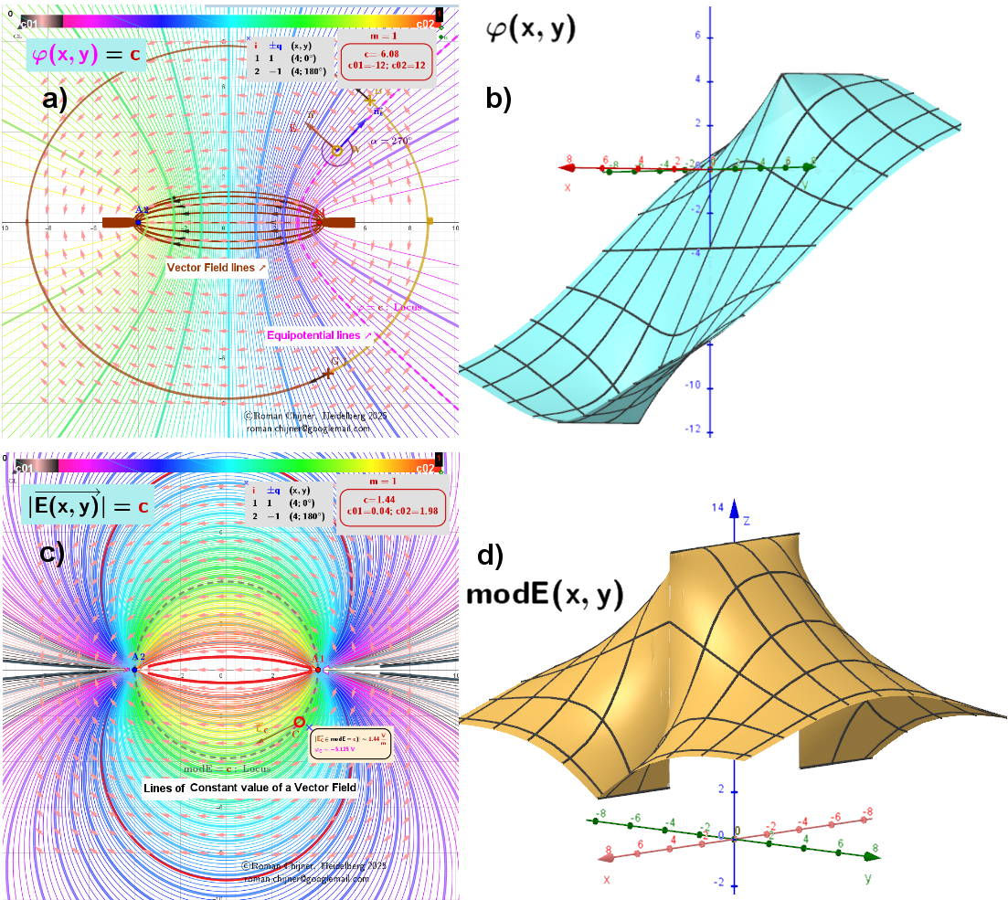
+ -. Visualization of scalar and vector fields of system of two positive point charges. The generalized potential function has the form φ(r)=Σqₖ*|rₖ –r|ᵐ, where m is a real number
[size=85] The images below were created using an [url=https://www.geogebra.org/m/yctnhz5a#material/msrrjbdv]applet[/url]. [/size][br][size=85] [size=85]This applet illustrates the construction of various scalar fields [b][color=#ff00ff]φ[/color][/b] for the selected parameters m=-1,1,0.4 and the corresponding gradient vector fields [b]E[/b] using the example of a [i]two-point system of identical 'charges'[/i] (designated as '++') located at a certain distance from each other.[/size][br] [b] The images below show[/b]:[br][color=#001d35][i]M[/i][/color][color=#001d35][i]ultifocal loci of points with: [/i][/color][br][color=#001d35]a) [/color][color=#001d35]equipotential lines [/color][color=#ff00ff][b]φ[/b][/color][color=#001d35][b]=[/b][/color][color=#ff0000][b]c [/b][/color][color=#001d35]and [/color][color=#980000]l[/color][color=#980000]ines [/color][color=#000000]of the corresponding gradient vector field[/color][color=#001d35][b]E[/b][/color][color=#001d35];[/color][br][color=#001d35]c) lines of equal field strength [/color][color=#001d35][b]modE(x,y) =[/b][/color][color=#ff0000][b]c[/b][/color][color=#000000][b].[/b][/color][br][i]Graphs of distribution functions in the xy-plane:[/i][br]b) potential -[b]φ(x, y)[/b];[br]d) values of the vector field -[b]modE(x,y)[/b].[br] Note that the gradient field lines are perpendicular to the equipotential lines.[/size]
m=-1. This is the case for a Coulomb or gravitational field.
m = 1. N-Ellipse - The case of multifocal curves (N≥2), the construction of which is a generalization of the construction of an ellipse-hyperbola.
m=0.4