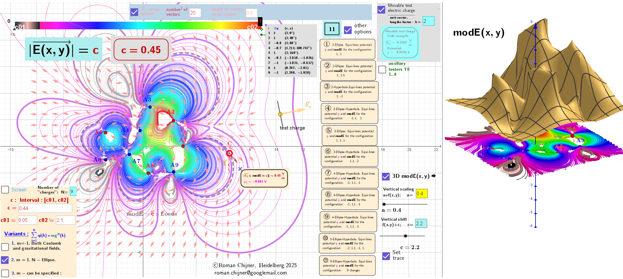
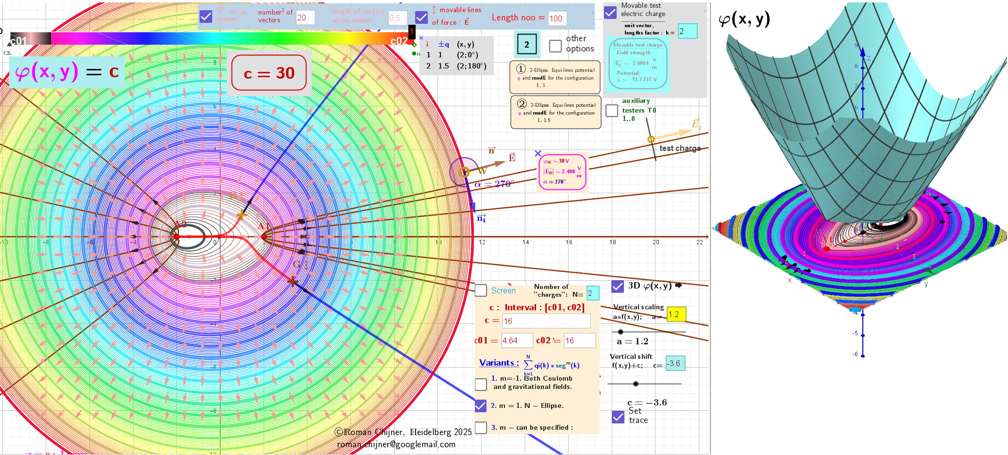
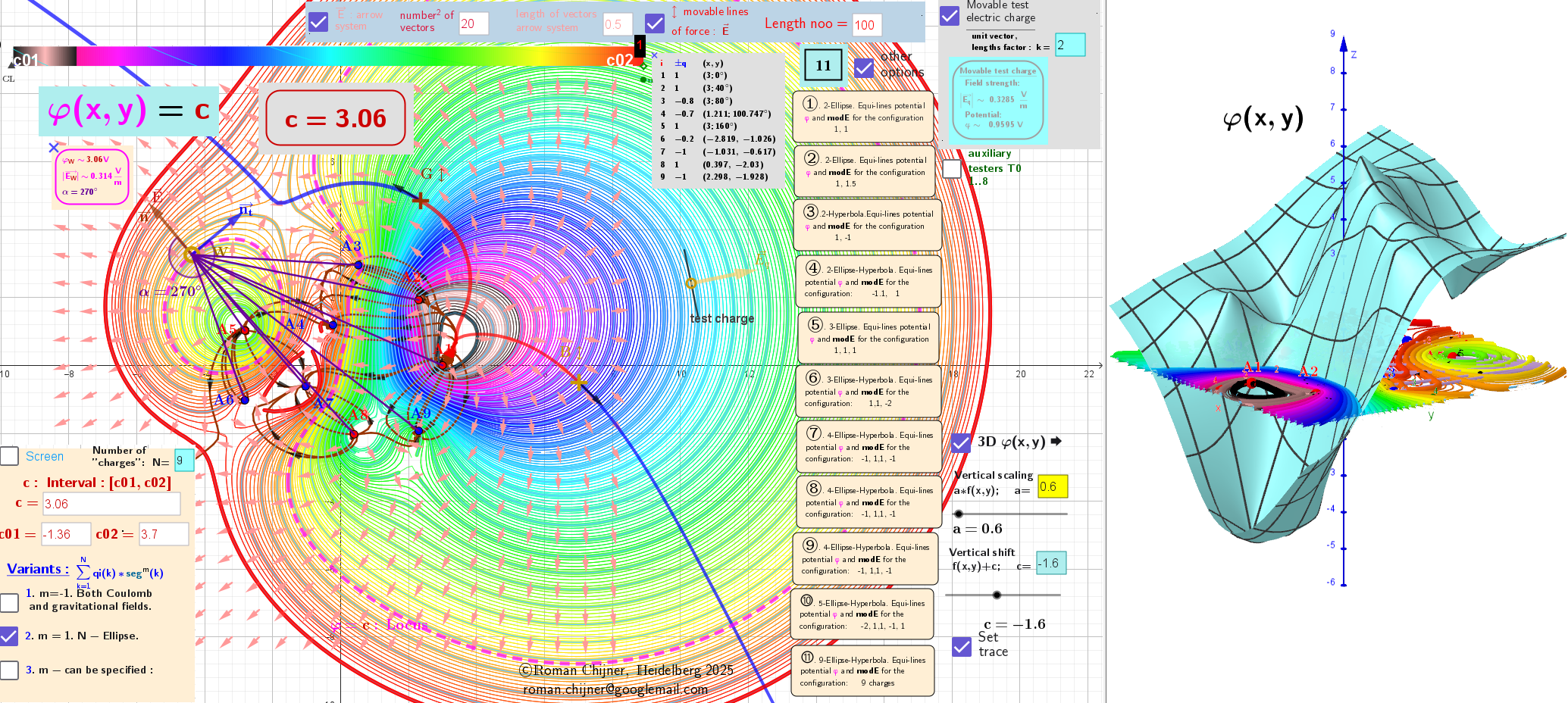
[size=85] The images below were created using an [url=https://www.geogebra.org/m/yctnhz5a#material/msrrjbdv]applet[/url]. The following explanations will help you to understand the images.[br]Two types of loci are calculated for [i]each combination of charges[/i]. Multifocal closed curves are constructed as follows:[br] 1. [color=#333333]The [b]first case [/b]corresponds to equipotential lines[/color], [b][color=#ff00ff]φ[/color] [/b]=[b][color=#980000]c[/color][/b], and the[br] 2. [color=#333333]The [b]second case [/b]corresponds to [/color]lines of equal values of the vector field, [b]modE[/b]= [color=#980000][b]c[/b][/color].[br] The variable [b][color=#980000]c[/color] [/b]lies within the interval [b][color=#980000]c[/color][/b]∈[[b][color=#980000]c₀₁[/color][/b],[b][color=#980000]c₀₂[/color][/b]], and the boundaries are set [i]manually [/i]so that all curves lie within the observation area. [br] The [b]Heatmap [/b]in contour diagrams visualizes the distribution of potential [b][color=#ff00ff]φ[/color] [/b](in case 1) and for the field [b]E [/b]-value [b]modE [/b](in case 2).[br][br]Each case is supported by two images a) and b).[br]1. [b]For the first case:[/b][br]a) [u]Contour diagram[/u]. Equipotential lines (closed curves of [color=#ff00ff][b]locus[/b] [/color][b][color=#ff00ff]φ[/color] = [color=#980000]c[/color][/b]). [i][color=#ff7700]For a gradient field, these lines are always perpendicular to the vector field lines [b]E[/b][/color].[/i] The directions of the vector field at each point in the field are shown by arrows and [color=#980000][i][b]vector field lines[/b][/i][/color] [color=#333333]drawn[/color] around each charge. [br](b) The potential [b]φ(x, y)[/b] is represented in three-dimensional space, where positive height corresponds to positive potential [b][color=#ff00ff]φ [/color][/b]and negative height corresponds to negative potential.[br]2. [b]For the second case:[/b][br]a) [u]Contour diagram[/u]: Lines of constant field value (closed curves of the [b]locus[/b] [b]modE[/b] = [b][color=#980000]c[/color][/b]). The value of the vector field is the same on each curve, but the [i]directions[/i] are different.[br](b) The distribution of vector field values is represented as a [i][b]surface[/b][/i] [b]modE(x, y)[/b] in three-dimensional space.[/size]

[color=#980000][b]Figure 1: A linear chain of two "charges" of different magnitude but the same sign creates a vector field.[/b][/color]

[b][color=#980000] [b][color=#980000]Figure 2: [/color][/b]A system of nine "charges" of different magnitudes and signs creates a vector field.[/color][/b]