[size=85] Solving an implicitly defined plane curve means splitting it into separate "curve sections" for which [b][i]explicit[/i][/b] expressions of functional dependencies can be written. These may take the form of analytical function definitions, y = f(x), or parametrically defined curves where the x-coordinate coincides with the parameter, x = t.[br] The [url=https://www.geogebra.org/m/kxyugn8n]applet [/url]considers the case of the [url=https://en.wikipedia.org/wiki/Trifolium_curve]Trifolium curve [/url]where an implicit equation of a plane curve is given in the form of a [i]biquadratic equation[/i] in the variable [b]y[/b]. Using its root formulas,[i] 4 explicit functional dependencies[/i] of the real variable [b]x[/b] are found that make up the plane curve under consideration. However, this method is not always applicable.[br] [b] This applet illustrates[/b] the use of the [i]method of parametrically defined complex functions[/i] to solve [b]the same implicit [i]biquadratic equation[/i][/b] in [b][color=#1e84cc]y[/color][/b]: [b][color=#1e84cc]eq[/color][/b]: [color=#1e84cc]x⁴ + 2x² [b]y²[/b] + a [b]y⁴[/b] - x³ + 3x [b]y²[/b] = 0[/color] . In the complex plane the variable [b][color=#1e84cc]x[/color][/b]→[b][color=#1e84cc]z[/color],[/b] [b][color=#1e84cc]y[/color][/b]→[b][color=#1e84cc]f(z)[/color][/b]. The [url=https://eqworld.ipmnet.ru/en/solutions/ae/ae0104.pdf]root formulas[/url] used are easily extended to the complex plane in a [url=https://www.reddit.com/r/geogebra/comments/1k35f1x/the_calculation_of_complex_numbers_in_algebra_is/]certain way[/url]. Roots: complex functions [b][color=#ff00ff]g1(z)[/color][/b],[color=#ff7700][b] g2(z)[/b][/color], [b][color=#0000ff]g3(z)[/color][/b] and [b][color=#38761d]g4(z)[/color][/b] are solutions of the corresponding complex equation.[br] Each of these functions f[b](z)[/b] has surfaces with [b]real[/b] and [b]imaginary[/b] parts ([b]Fig. 1)[/b]. In the problems considered, however, their values are only [b]in the plane y=0[/b] along the real [b]x-Axis[/b] on the interval [a1,a2], where the imaginary part is zero. [b][color=#f4cccc]Curve(a,real(f(z)),a,a1,a2)[/color][/b][color=#f4cccc],[/color] where [b][color=#e69138]Curve(a,imaginary(f(z)),a1,a2)=0[/color][/b], is the part of the original plane curve on this interval. See the images [b]Fig. 2[/b] below the applet.[br] [br]*[url=https://www.geogebra.org/m/kxyugn8n]Previous applet[/url]: Finding explicit expressions of four real functions for an implicitly defined plane curve whose equation is biquadratic in the variable [b]y[/b].[/size]
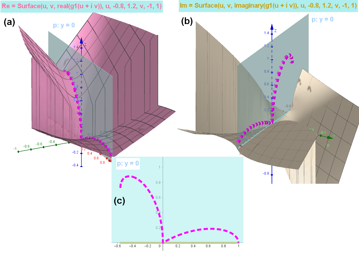
[size=85][b]Fig. 1:[/b] [b]Surfaces of the [color=#ea9999]real[/color] [color=#ea9999]part[/color] (a) and the [color=#ff7700]imaginary part[/color] (b) of [color=#ff00ff]g1(z)[/color] over the the complex plane. [/b][br] To determine the branch of a plane curve given by an [i]implicit equation[/i], it is necessary to consider the behavior of these surfaces [b]in the plane y=0 (c)[/b], in particular on the interval where the [b][b]imaginary[/b] [/b]part of [b]g1(z)[/b] [i]is zero[/i], and its [b]real[/b] part is the [color=#ff00ff][b]desired part of the curve[/b][/color].[/size]
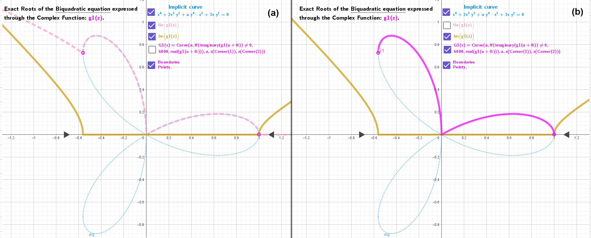
[size=85][b] [b] Fig. 2: The behaviour of [color=#ff00ff]g1(z)[/color] in the y=0 plane.[/b][br] (a)[/b][b] ●The curve [/b][color=#f4cccc]Re(g1(z))[/color][b][color=#f4cccc]=Curve(a, real(g1(a + 0ί)), a, x(Corner(1, 1)), x(Corner(1, 2))) [/color][/b][b]-the real[/b][b] part [/b][b]of the complex function: Re[/b][b]( g1(z)[/b][b] ) is plotted as a dashed, [/b][color=#f4cccc]light purple[/color][b] curve. [br] ●The [color=#333333]curve[/color][color=#e69138] Im(g1(z))=Curve(a, imaginary(g1(a + 0ί)), a, x(Corner(1, 1)), x(Corner(1, 2)))[/color][/b][b] -the imaginary part [/b][b]of the complex function: Im[/b][b]( f1(z)[/b][b] ) is plotted as a solid [color=#e69138]Chinese Gold[/color][/b][b] color curve.[br] (b) [/b][color=#ff00ff][b]G1(x)[/b][/color][b][color=#ff00ff]= Curve(a, If(imaginary(g1(a + 0ί)) ≠ 0, 6000, real(g1(a + 0ί))), a, x(corner(1)), x(corner(2)))[/color][/b][b] - is the [i]resulting curve[/i][/b][b]. Shown as a solid [/b][color=#ff00ff][b]magenta[/b][/color][b] line.[br] From the comparison of images (a)[/b][b] and (b)[/b][b] it is clear that [/b][i]from the whole dashed [b][color=#f4cccc]light purple[/color][/b] curve[/i][color=#f4cccc][b] Re(g1(z)) [/b][/color][i]only the part in the region where [color=#e69138][b]Im(g1(z))[/b][/color][b]= 0[/b][/i][b] is [i]cut out[/i][/b][b] and [i]kept.[/i][/b][/size]