[size=85][i] A [/i][url=https://en.wikipedia.org/wiki/Generalized_conic]multifocal oval[/url][i] is a curve defined as the [/i][b]locus[/b][i] of a point A([b]r[/b]) that moves in such a way that the [/i][b][color=#0000ff]sum of the distances [/color][/b][color=#ff00ff][b]φ[/b][/color][i]([b]r[/b]) [b][color=#0000ff]to[/color][/b] [/i][b]n[/b][i] [b][color=#0000ff]points[/color][/b] remains constant. It is also known as a [/i][url=https://mathcurve.com/courbes2d.gb/multiellipse/multiellipse.shtml][color=#ff7700]Multifocal Ellipse[/color][/url][i] ([/i][url=https://en.wikipedia.org/wiki/N-ellipse][color=#980000][i]n[/i]-ellipse[/color][/url][i]) with [/i][b]n [/b][b][color=#ff0000]foci[/color][/b][i] (or [b]n[/b] poles).[br] The potential function [b][color=#ff00ff]φ[/color][/b]([b]r[/b]) is generalized by this applet to generate the corresponding multifocal curves.[br] [/i][size=85][i][i][i][i][i][i][i][i][i][b][i][i][i][b][i][b][i][b][b][i][color=#767676]The [/color][color=#0000ff]sum[/color][color=#0000ff] o[/color][color=#0000ff]f t[/color][size=85][color=#0000ff]he m-th powers of the distances [/color][color=#0000ff]to [/color][color=#333333]n[/color][color=#0000ff] points[/color][color=#333333] is given here by [/color][/size][/i][/b][/b][/i][/b][/i][/b][/i][/i][/i][/b][/i][/i][/i][/i][/i][/i][/i][/i][/i][color=#0000ff][color=#0000ff][color=#0000ff][size=85][color=#ff00ff][b]φ[/b][/color][color=#333333][b](r)=[/b][i][i][i][i][i][i][i][i][b]Σqₖ*|rₖ–r|ᵐ[/b][/i][/i][/i][/i][/i][/i][/i][/i], where k=1..[b]n[/b] and [b]m∈ℝ[/b]. [b]qₖ[/b] - weight factors, which here, by analogy with electromagnetism, we will call "charges". [/color][/size][/color][/color][/color][/size][br][i][br] ●The purpose of the applet is to visualise [/i][url=https://mathcurve.com/courbes2d.gb/orthogonale/orthogonale.shtml]double orthogonal systems[/url][i] for [/i][color=#9900ff]scalar[/color][i] functions of the above type. In particular: [/i][i]for [/i][b]m[/b][i] = -1, this is the well-known result in electromagnetism that electric [/i][color=#980000]field lines[/color][i] and [/i][color=#ff00ff]equipotential lines[/color][i] form a double orthogonal system. For [b]m[/b]=1 -[url=https://en.wikipedia.org/wiki/N-ellipse][i]n[/i]-ellipse[/url] , [b]m[/b]=2 - [url=https://www.geogebra.org/material/show/id/arrctwvn]case[/url]. [br]●The applet constructs [/i][b]loci[/b][i]. For a [color=#9900ff]given [url=https://www.google.com/search?q=what+Scalar+field&sca_esv=b3f6a4e4ace9f962&rlz=1C1VDKB_deDE963DE963&sxsrf=AE3TifNaeH1mlgh2NkZ_lPDl2gyWT2xiLg%3A1752848303285&ei=r1d6aLOYEYmrxc8PkrqOoAs&ved=0ahUKEwjzq9njzMaOAxWJVfEDHRKdA7QQ4dUDCBA&oq=what+Scalar+field&gs_lp=Egxnd3Mtd2l6LXNlcnAiEXdoYXQgU2NhbGFyIGZpZWxkMgYQABgHGB4yBhAAGAcYHjIGEAAYBxgeMgYQABgHGB4yBhAAGAcYHjIGEAAYBxgeMgYQABgHGB4yBhAAGAcYHjIGEAAYBxgeMgYQABgHGB5I9DRQqRNYyydwAXgBkAEAmAFxoAGDBKoBAzIuM7gBDMgBAPgBAZgCBqAClQTCAgoQABiwAxjWBBhHwgINEAAYgAQYsAMYQxiKBcICBxAAGIAEGA2YAwCIBgGQBgqSBwMzLjOgB-ousgcDMi4zuAeQBMIHBTAuNS4xyAcP&sclient=gws-wiz-serp]scalar field[/url] [/color][/i][color=#ff00ff][b]φ[/b][/color][i](r), it creates [br][/i][color=#ff00ff]-equipotential lines[/color][i], and for the corresponding gradient fields [/i][b]E[/b][i](r), it creates [br]-iso-magnitude lines, which are lines of constant field magnitude ([/i][color=#1e84cc]but not their direction![/color][i]), denoted by [/i][b][color=#333333][url=https://www.google.com/search?sca_esv=9df8d0d36b3fc424&rlz=1C1VDKB_deDE963DE963&sxsrf=AE3TifOinHFuIQvbGNLrnpGmgfmwCNS3IQ:1751026231589&q=what+is+Equi-lines+potential+%CF%86+and+modE&spell=1&sa=X&ved=2ahUKEwjMxZqEyZGOAxW_FBAIHQEZGxMQBSgAegQICxAB]modE[/url][/color]. [/b][i]The vector field [/i][b]E[/b][i](r) is obtained by taking the[/i][b][color=#980000] [url=https://en.wikipedia.org/wiki/Gradient]gradient[/url] [/color][/b][i]of the potential function [color=#ff00ff][b]φ[/b][/color](r)[/i][i].[br]● For a set of point "charges", these [/i][b]loci[/b][i] are always closed, and the "charges" are their [/i][b][color=#ff0000]foci[/color][/b][i]. In other words, these lines are multifocal curves[/i][i].[br]● [/i][color=#ff00ff]Equipotential lines[/color][i] are [/i][color=#333333][i]always perpendicular [/i][/color][i]to the [color=#980000]field lines[/color][/i][i] of the [/i][url=https://en.wikipedia.org/wiki/Conservative_vector_field]conservative[/url][i] vector field [/i][b]E[/b][i](r), which are calculated numerically in the applet.[br][/i][/size] [size=85]Description of Services of this applet you will find in [url=https://www.geogebra.org/m/adevardg ]1[/url], images of examples in [url=https://www.geogebra.org/m/vvqwdngb ]2[/url], [url=https://www.geogebra.org/m/htxqtc5v ]3[/url], [url=https://www.geogebra.org/m/qqbbe28g]4[/url], [url=https://www.geogebra.org/m/hzsb6a5p ]5[/url], [url=https://www.geogebra.org/m/yjtysjma ]6[/url], [url=https://www.geogebra.org/m/wd2bxbd6 ]7[/url], [url=https://www.geogebra.org/m/remwjr7t ]8[/url], [url=https://www.geogebra.org/m/ygtcty7y ]9[/url].[/size]
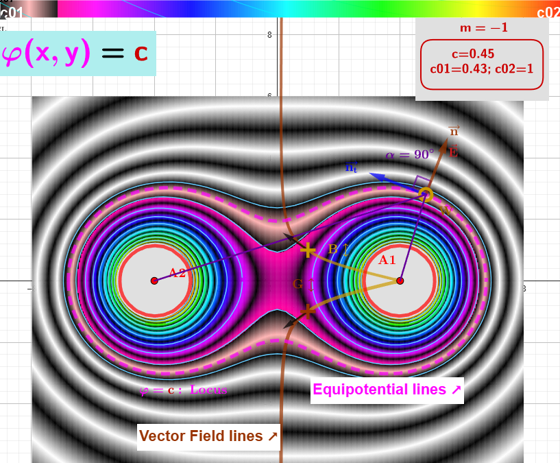
[size=85] The Heatmap, created by scanning outside parameter [b][color=#980000]c∈[c01,c02][/color][/b], draws black and white curves.[/size]
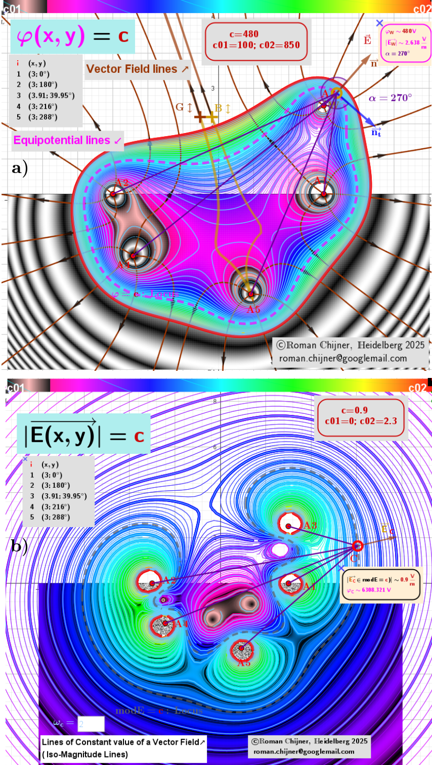
[b][color=#980000]Examples of five charges [/color][/b]
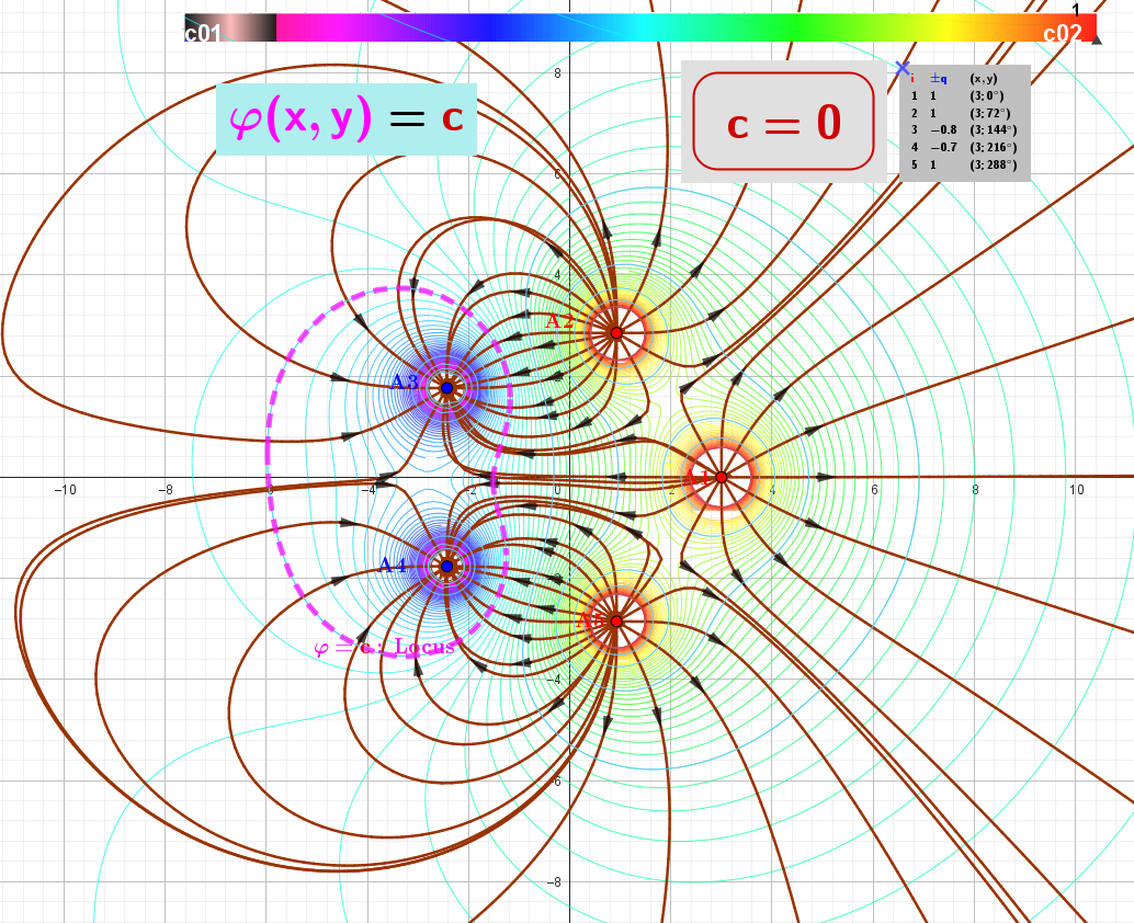
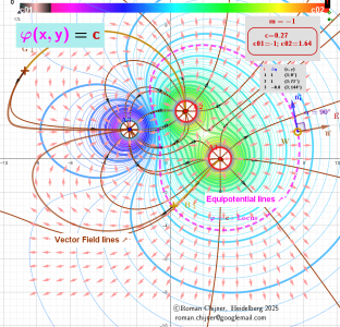
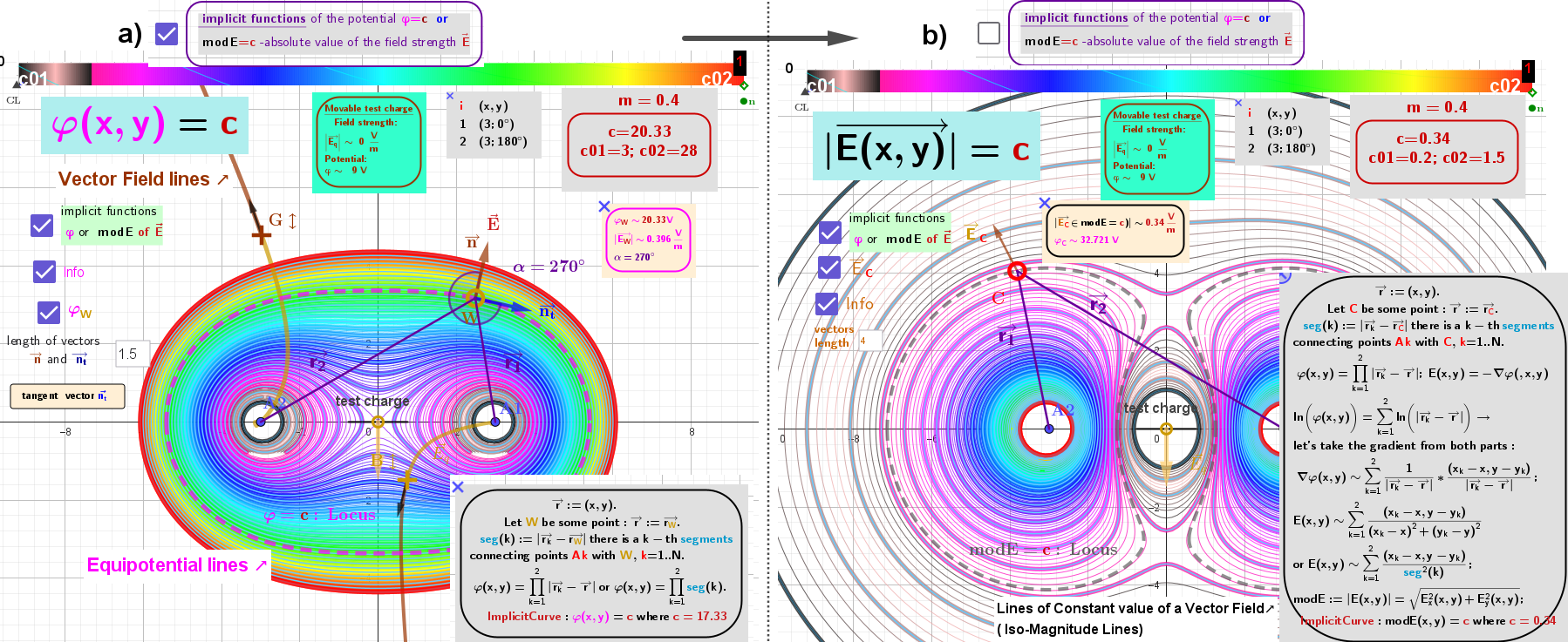
[size=85][b][color=#333333]Figure 1:[/color][/b][color=#333333]The [/color][i][b][color=#ff00ff]equipotential lines[/color][/b][/i][color=#333333] of a scalar field [/color][b][color=#ff00ff]φ [/color][/b][color=#333333]are always perpendicular to the [/color][i][color=#980000][b]lines of force[/b] [/color][color=#333333]of the corresponding gradient field [/color][/i][b]E[/b][color=#333333]. [/color][br][/size]
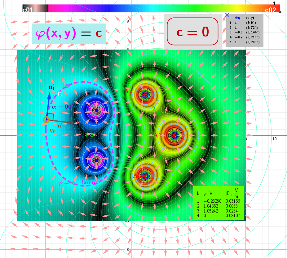
[size=85][b]Figure 2: [/b][color=#333333]The [/color][b]Heatmap [/b][color=#333333]showing the distribution of the scalar field [/color][b][color=#ff00ff]φ[/color][/b][color=#333333] around the charges, along with the directions of the corresponding gradient vector field [/color][b]E[/b][color=#333333], is depicted as [/color][b][color=#ea9999]arrows[/color][/b][color=#333333]. Here the [/color][b][color=#ff00ff]Equipotential lines[/color][/b][color=#333333] of the scalar field [/color][b][color=#ff00ff]φ[/color][/b][color=#333333] are closed curves whose [/color][b][color=#ff0000]foci[/color][/b][color=#333333] are located on the charges.[/color][/size]
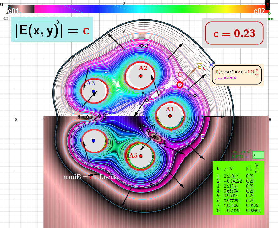
[size=85][b][color=#333333]Figure 3[/color][color=#980000]: [/color][/b]The [b]Heatmap[/b] and [b]Contour lines[/b] shows the distribution of the [i]constant value of the vector field strength modulus[/i] [b]E[/b] for five point charges (denoted [b]modE[/b]). In this case, the [i]lines representing the constant value of the vector field strength[/i] modulus [b]E[/b] (but not their directions!) always form closed curves, the [b]foci[/b] of which are[i] located at the charges[/i].[br][/size] [size=85]The table shows the values of the potential [b][color=#ff00ff]φ[/color][/b] and [b]modE[/b] at test points 1–6, which are located on the locus [b]modE[/b]=[color=#980000][b]c[/b][/color]. Test points 7 and 8 are at points where the field [b]E[/b] is almost zero.[/size]