
Equations of branches of implicitly defined curves
[b]Statement of the problem:[/b] The curve is given in implicit form as g(x, y) = 0, for example a circle as y² + x² = 1. [b]Find[/b]: the explicit form of the equations y=f(x) for each of the k branches of the curve, i.e. {fᵢ(x)}, where i=1..k. For a circle, for example, f₁(x) = sqrt(1-x²) for y > 0, and f₂(x) = − sqrt(1-x²) for y < 0. If f(x, y) is a quadratic function with respect to variable y, GeoGebra can easily find the roots in symbolic form, y₁(x) and y₂(x). For polynomials of the 3rd and 4th degree, knowing the existing rigorous [url]https://www.geogebra.org/m/v4fvf8nx[/url] of their equations in symbolic form, one can find the equations of the branches {fᵢ(x)} of the corresponding plane curves using complex functions.
Table of Contents
- Multifocal plane curves
- Ellipses and Hyperbolas defined geometrically as locus of points
- Cassini ovals and their orthogonal trajectories (hyperbolas)
- What is the Locus of a point that moves in such a way that it's sum of the squares of the distance (with weight factors) to N fixed points remains constant?
- Construction of multifocus curves, whose locus is relative to |x - xᵢ| - distances of some selected points - foci, having the given conservation properties of some selected value
- 1. Images of the construction of multifocal curves corresponding to the potential lines of the electrostatic field
- 2. Images of the construction of multifocal curves corresponding to "potential lines"-Contour lines for various "charge" configurations of n-ellipse/hyperbola
- 3. Images of the construction of multifocal curves corresponding to "potential lines"-Contour lines for various "charge" configurations of n-Lemniscate
- Biquadratic equation
- Finding explicit expressions of four real functions for an implicitly defined plane curve (Trifolium curve) whose equation is biquadratic in the variable y
- Branches of an implicitly defined biquadratic curve found using complex functions: Trifolium curve
- Branches of an implicitly defined biquadratic curve found using complex functions: Cartesian oval
- Images: Branches of an implicitly defined biquadratic curve found using complex functions: Cartesian oval
- Examples of finding the equations of branches of implicitly defined cubic curves
- An example of finding explicit equations for curves using complex functions that make up an implicitly defined cubic curve
- Images: An example of finding explicit equations for curves using complex functions that make up an implicitly defined cubic curve
- Examples of an implicit equation of a plane curve of the quartic equations
- An example of finding explicit equations for curves using exact roots as complex functions that make up an implicitly defined quartic plane curve whose equation has 15 coefficients
- Images. An example of finding explicit equations for curves using exact roots as complex functions that make up an implicitly defined quartic plane curve whose equation has 15 coefficients
- Examples of implicit equations of a plane curve of third-degree equations
- Mapping Focal Branches via Implicit Equations: The Half-Wave Zone Slit Model
Ellipses and Hyperbolas defined geometrically as locus of points
Inspired by material from Wikipedia: [url=https://en.wikipedia.org/wiki/Ellipse#Definition_as_locus_of_points]Ellipse[/url] and [url=https://en.wikipedia.org/wiki/Hyperbola#As_locus_of_points]Hyperbola[/url] as locus of points. [br]
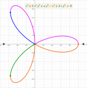
Finding explicit expressions of four real functions for an implicitly defined plane curve (Trifolium curve) whose equation is biquadratic in the variable y
[size=85]x⁴ + 2x² [b]y²[/b] + a [b]y[/b]⁴ - x³ + 3x [b]y²[/b] = 0 [br] Biquadratic equation, the solution [b]y[/b]=y([b]x[/b]) of which is found by the formulas[url=https://eqworld.ipmnet.ru/en/solutions/ae/ae0104.pdf] EqWorld[/url]. The branches of the implicit function generally correspond to the real functions f(x) on the considered domains of definition of the implicit function.[br] The vertical asymptotes are found using the [url=https://en.wikipedia.org/wiki/Implicit_function_theorem]implicit function theorem[/url] and the calculations are done in CAS.[br] *Following [url=https://www.geogebra.org/m/kwdbdznt]applet[/url]: Branches of an implicitly defined biquadratic curve found using complex functions.[/size]
An example of finding explicit equations for curves using complex functions that make up an implicitly defined cubic curve
[size=85][u][b]Statement of the problem:[/b][/u][br]The curve is given in [b]implicit[/b] form as g(x, y) = 0, for example a circle as y² + x² = 1.[br][u][b] Find:[/b][/u][br]the [b]explicit [/b]form of the equations y=f(x) for each of the [b]k[/b] branches of the curve, i.e. {f[b]ᵢ[/b](x)}, where i=1..k. For a circle, for example, f₁(x) = sqrt(1-x²) for y > 0, and f₂(x) = − sqrt(1-x²) for y < 0. If f(x, y) is a quadratic function with respect to variable [b]y[/b], GeoGebra can easily find the [b]roots [/b]in symbolic form, y₁(x) and y₂(x).[br] For polynomials of the 3rd and 4th degree, knowing the existing rigorous [url=https://www.geogebra.org/m/v4fvf8nx][u][b]solutions[/b][/u][/url] of their equations in symbolic form, one can find the equations of the branches {f[b]ᵢ[/b](x)} of the corresponding plane curves using complex functions.[br] Earlier, I considered biquadratic equations for the [url=https://www.geogebra.org/m/kwdbdznt][u][b]Trifolium curve[/b][/u][/url] and the [url=https://www.geogebra.org/m/cgfbcxau][u][b]Cartesian oval[/b][/u][/url]. These examples illustrate the application of complex functions. In these cases, it is possible to find the equations of the branches of curves using both [i][b]real functions[/b][/i] and [i][b]complex functions[/b][/i], from the real part of the functions of which only those sections are left where the corresponding complex part is missing, i.e. Im(x)=0.[br][/size][size=85] This applet considers an example from mathstackexchange: [url=https://math.stackexchange.com/questions/3980344/branches-of-implicitly-defined-cubic-curves]Branches of implicitly defined cubic curves[/url] for an implicitly defined cubic curve [b]a y³ + b y² + c y + d(x) = 0 where d(x)=-5 x³ + x² + 45x - c0[/b], for which I found explicit equations of the curves of its branches using complex functions.[br] Images of three examples are in the [url=https://www.geogebra.org/m/rek5mz4n]applet.[/url][/size]
An example of finding explicit equations for curves using exact roots as complex functions that make up an implicitly defined quartic plane curve whose equation has 15 coefficients
[size=85] This applet illustrates an example of finding equations of branches of a plane curve of degree four (specified implicitly) using existing[b][url=https://www.geogebra.org/m/v4fvf8nx] rigorous solutions[/url][/b] in the form of complex functions in symbolic form.[br] The [b] [url=https://en.wikipedia.org/wiki/Quartic_plane_curve]Quartic plane curve[/url] [/b]of the [b]fourth order [/b]has 15 coefficients: A [b]x[/b][sup][b]4[/b][/sup]+B [b]y[sup]4[/sup][/b]+C [b]x[sup]3 [/sup]y[/b]+D [b]x[sup]2 [/sup]y[sup]2[/sup][/b]+E [b]x y[sup]3[/sup][/b]+F [b]x[sup]3[/sup][/b]+G [b]y[sup]3[/sup][/b]+H [b]x[sup]2 [/sup]y[/b]+I [b]x y[sup]2[/sup][/b]+J [b]x[sup]2[/sup][/b]+K [b]y[sup]2[/sup][/b]+L[b] x y[/b]+M[b] x[/b]+N [b]y[/b]+P=0, where at least one of A, B, C, D and E is non-zero. You can explore these curves by adjusting the coefficients using the sliders.[br] Images of three examples are presented in the [url=https://www.geogebra.org/m/wmwsrksg]applet[/url][b].[/b][br][/size]
Mapping Focal Branches via Implicit Equations: The Half-Wave Zone Slit Model
[size=85][b] Applet Description: Focal Curves in Near-Field Slit Diffraction[br][/b]This applet derives [b]explicit equations[/b] for the focal curves within the [b]Half-Wave Zone [url=https://www.geogebra.org/m/n62bumu7]Model[/url][/b] of slit diffraction.[b][br]1. Visualization of Stationary Points[br][/b]The ap plet identifies the stationary points of the 2D distribution J(x, y) using a distinct color-coded system:[br][list][*][b]Red & Blue Points:[/b] Represent local [b]maxima[/b] and [b]minima[/b], respectively.[br][/*][*][b]Crosses (Multiple Colors):[/b] Represent [b]saddle points[/b] positioned between the extrema.[br][/*][*][b]Symmetry:[/b] Note that the distribution of these points is symmetric with respect to the y-axis.[/*][/list][b][br]2. From Implicit Equations to Cubic Roots[br][/b]The derivation begins with the implicit equation ([b][url=https://www.geogebra.org/m/qgg4ujte]eq00[/url][/b]) for the focal curves. By eliminating irrational terms, this is transformed into a [b]cubic polynomial equation[/b] ([b][url=https://www.geogebra.org/m/a8h6psbh]eq0[/url][/b]).[br]We solve the general cubic form: a(z)y[sup]3[/sup] + p(z)y[sup]2[/sup] + c(z)y + d(z) = 0[br]where z is treated as a complex variable. This allows us to express the roots in the explicit form y = f(z). All [url=https://www.geogebra.org/material/show/id/v4fvf8nx]symbolic[/url] and numerical computations were performed directly within [b]GeoGebra[/b].[br][b][br]3. Analysis of the Solution Branches[/b][list][*][b]Curve Cu[sub]f1[/sub]:[/b] Corresponds to the real part of the first complex function, f1(z). This branch coincides perfectly with the original implicit function [b]eq00[/b].[/*][*][b]Curve Cu[sub]f2[/sub][/b],[b][sub] [/sub][/b][b]Curve Cu[sub]f3[/sub][/b] [b]:[/b] Correspond to the real part of the complex functions f2(z), f3(z), respectively, and represent subsequent transformations and additional branches of the cubic solution.[br][/*][/list][quote][b][/b][b]Notes:[/b] [br] Rendering complex functions is computationally intensive. Please be patient or use a desktop computer for a smoother experience.[br] Below the applet, you will find images of the CAS transformations and the behavior of the curves related to the solutions f1(z), f2(z), and f3(z).[/quote][/size][quote][/quote]
Obtaining the implicit equation (eq00) of the focal curve:
Obtaining the implicit equation of the focal curve (eq0) from the equation (eq00) by eliminating irrationality from it:

1. The transformation to eliminate irrationality in the focal curve introduces additional branches to the implicit function

[size=85][b]Implicit functions before (a) and after (b) transformation.[/b] As illustrated in the secondary plot, the transformation to eliminate irrationality in the focal curve introduces additional branches to the implicit function.[/size]
2. Branches of the complex solutions for the cubic polynomial

[size=85](a) The implicit function following transformations, reduced to a cubic polynomial form.[br][br](b)–(d) Branches of the complex solutions for the cubic polynomial. As illustrated, the [i]imaginary components[/i] of these complex solutions vanish along the [i]real [/i]axis.[br] While the first branch, [color=#ff0000][b]f1(z)[/b][/color], satisfies the [color=#0000ff][b]original implicit function[/b][/color], the remaining two branches emerge as a result of the subsequent transformations.[/size]